Understanding Word2Vec and Paragraph2Vec

In these notes we compute the update steps for Para2Vec algorithm (Le & Mikolov, 2014). These notes focus on the Distributed Memory (dm) model with mean taken at hidden layer (DM-mean). The original paper describes several other variants.Para2Vec is an adaptation of the original word2vec algorithm, the update steps are an easy extension.

1. Word2Vec

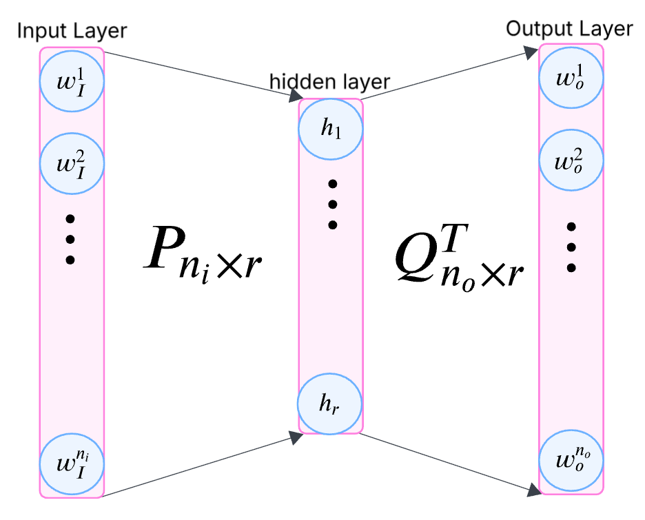
We start by looking at the word2vec continuous bag of words model, with negative sampling and mean taken at hidden layer. This is a single hidden layer neural network.

Notation

Let $W_I = \lbrace{ w_I^0,\,w_I^1,\,\ldots\,w_I^{n_i}\rbrace}$ and $W_O= \lbrace{ w_O^0,\,w_O^1,\,\ldots\,w_O^{n_o}\rbrace}$ denote the set of input and output layer nodes respectively. Let $h$ denote the vector at the hidden layer. $n_i \,=\, |W_I|$, $r$, $n_o \,=\,|W_O|$ represent the size of input, hidden and output layer respectively. Let $p_i \in \mathbb{R}^r$ and $q_j \in \mathbb{R}^r$ be the vector representation of the $i^{th}$ input and $j^{th}$ output node respectively. Let $P$ represent a matrix of input layer weights with $i^{th}$ row vector as $p_i^T$ and similarly matrix $Q$ is also defined.

Training

The training set consists of pair of context-target entities. Context entities (set of words in word2vec, documents and words in doc2vec) are used to predict the target entity at output layer. Let $\mathcal{C}$ and $\mathcal{T}$ represent the set of context and target entities respectively.

For a given training sample, let $C=\lbrace{ w_I^{c_1},\ldots \, w_I^{c_{\lvert C \rvert } }\rbrace}$ represent the sequence of $|C|$ context entities and $W_O^{j^*}$ be the target entity. Word2Vec training maximizes the conditional probability of the target given the context. This probability is modeled using softmax function as:

\[P(W_O^{j^*}|C) = \frac{\exp({q_{j^*}}^Th)}{\sum_j^{n_o}\exp({q_{j}}^Th)}\]

where $h$ is constructed in a feed-forward manner as

\[h = \frac{1}{|C|} \sum_{i\in {C}} p_{i}\]

To compute the update, we take a step in the direction of gradient of $ \log P(W_O^{j^*}|C )$. Let \(f(q_{0},\,\ldots,\,q_{n_o},h) \,=\,\log(P(W_O^{j^*}|C))\)

\[\frac{\partial f}{\partial q_{i}} = \left(I(i=j^*)- \frac{\exp({q_{i}}^Th)}{\sum_j^{n_O}\exp({q_{j}}^Th)}\right)h = \left(I(i=j^*)- P(w_O^{i}|C)\right)h = e_i h\]

where $e_i = \left(I(i=j^*)- P(q_i|C)\right)$ denotes the error incurred at $i^{th}$ output node.

At $(t+1)^{th}$ step:

\[q_i^{t+1} \leftarrow q_{i}^t + \eta e_i h\]

Further, note that

\[\frac{\partial f(q_0,\,\ldots,\,q_{n_o},h)}{\partial p_i} = \sum_j^{n_o} \frac{\partial f}{\partial q_j} \frac{\partial q_j}{\partial p_i} + \frac{\partial f}{\partial h} \frac{\partial h}{\partial p_i}\]

Note, $\frac{\partial q_{j}}{\partial p_{i}}\,=\, 0$ as $Q$ and $P$ are independent. Thus,

\[\frac{\partial f}{\partial p_{i}} = \frac{\partial f}{\partial h} \frac{\partial h}{\partial p_i} = \frac{1}{|C|} \frac{\partial f}{\partial h} \;\text{for}\;w_I^i \in \mathcal{C},\] \[\quad = 0 \; \text{otherwise}\]

where,

\[\frac{\partial f}{\partial h} = \sum_j^{n_o} (I(j=j^*)- P(w_O^{j}|C))q_j = \sum_j^{n_o} e_jq_j\]

Thus, update step for $p_{i}$ where $w_I^i \in \mathcal{C}$ is:

\[p_{i}^{t+1} \leftarrow p_i^t + \frac{\eta}{|C|} \sum_j^{n_o} e_j q_j\]

For $w_I^i \not \in \mathcal{C}$:

\[p_{i}^{t+1} \leftarrow p_i^t\]

Time Complexity of updates for every training sample

$P(w_O^{i}|C)$ computation at each output node requires $O(n_o)$ operations. The update equations above require $O(n_o r)$ computations. As $n_o$ can be in millions, this is prohibitive as we may have millions of words in the vocabulary. Negative sampling has been proposed as a potential solution to these scalability challenges.

Negative Sampling

The bottleneck step in previous computations is the softmax normalization. We can replace softmax by some other model, a commonly used one being logit/sigmoid function, defined as:

\[\sigma(x) = \frac{1}{1+e^{-x}}\]

Logit has range in $(0,1)$. It has some interesting properties:

\[\begin{align*} \frac{d\sigma(x)}{dx} &= \sigma(x)\sigma(-x)\\ \frac{d\log \sigma(x)}{dx} &= \sigma(-x) \\ 1-\sigma(x) &= \sigma(-x) \end{align*}\]

In softmax based approach we maximized the probability of target word conditioned on Context words. Note that as softmax is normalized, this also incorporates minimizing probability of non-target words. For negative sampling instead of considering all non-target words (also known as negative words), few examples are randomly sampled to constitute a negative sample set $\mathcal{N}$. The objective function for negative sampling becomes:

\[\max \; P(W_O^{j^*}|\mathcal{C})\Big(\Pi_{j\in\mathcal{N}} (1-P(W_O^{j}|\mathcal{C}))\Big)\]

where, $P(W_O^{j}|\mathcal{C}) = \frac{1}{1+e^{-q_j^Th}}$. Although we model the conditional probability as logit, it is not a well defined probability distribution as it isn’t normalized i.e. $\sum_j^{n_o} P(W_O^{j}|\mathcal{C}) \neq 1$. Goldberg–Levy explain a way to see the above objective function in terms of a well defined distribution.

Note that we could have also maximized a slightly different objective function: \(\frac{P(W_O^{j^*}\|\mathcal{C})}{\Pi_{j \in \mathcal{N}} P(W_O^{j}\|\mathcal{C})}\). We will later come back to this.

Derivation of update steps is similar to the softmax case:

\[f(q_{0},\,\ldots,\,q_{n_i},h) =\,\log\Big(P(W_O^{j^*}|\mathcal{C})\big(\Pi_{j\in\mathcal{N}} (1-P(W_O^{j}|\mathcal{C}))\big)\Big) = \log \sigma(q_{j^*}^Th) + \sum_{j\in \mathcal{N}}\log \sigma(-q_j^Th)\] \[\begin{align*} \frac{\partial f}{\partial q_{i}} &= (I(i=j^*) - \sigma(q_{j}^Th))h = (I(i=j^*)- P(w_O^{i}|C))h \\ &= e_i h \quad \forall i\in \mathcal{N}\,\cup\,\{ j^* \}, \\ &= 0 \; \text{otherwise} \end{align*}\]

where $e_i = (I(i=j^*)- P(w_O^i|C))$ denotes the error incurred at $i^{th}$ output node.

Update for output node vector thus is:

\[\begin{align*} & q_i^{t+1} \leftarrow q_{i}^t + \eta e_i h \quad i \in \mathcal{N}\,\cup\,\{ j^* \} \\ & q_i^{t+1} \leftarrow q_{i}^t \quad \text{otherwise} \end{align*}\]

For $p_i$:

\[\begin{align*} \frac{\partial f}{\partial p_{i}} &= \frac{\partial f}{\partial h} \frac{\partial h}{\partial p_i} = \frac{1}{|C|} \frac{\partial f}{\partial h} \;\text{for}\;w_I^i \in \mathcal{C}, \\ &= 0 \; \text{otherwise} \end{align*}\]

where,

\[\frac{\partial f}{\partial h} = \sum_j^{\mathcal{N}} \big(I(j=j^*)- \sigma(q_{j}^Th)\big)q_j = \sum_j^{\mathcal{N}} e_jq_j\]

Update for $p_i$ where $w_I^i \in \mathcal{C}$ is:

\[p_{i}^{t+1} \leftarrow p_i^t + \frac{\eta}{|C|} \sum_j^{\mathcal{N}} e_j q_j\]

Time Complexity of Negative Sampling

Computing updates above takes $O(|\mathcal{N}|r)$ time for output vectors and $O\big((|\mathcal{N}|\,+\, |\mathcal{C}|)r\big)$ for input vectors. As the number of negative samples and context words are small constants, this method is practically $O(r)$.

2. Paragraph2Vec

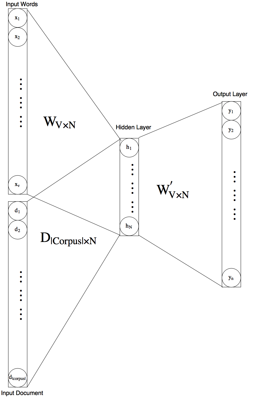
Paragraph2Vec technique includes several different algorithms. We discuss DM with average at hidden layer. The only difference from word2vec is inclusion of documents along with words as input nodes. P2V neural net has input nodes representing documents in the training data.

The rationale behind including documents as input nodes is based upon considering documents as another context. In this abstract sense of context there is no difference between a word and a document. At the time of training we consider (context set, target) pairs as in word2vec, however, for P2V document is also considered a member of the context set. The objective function and the training update steps are exactly the same as word2vec.

Inference

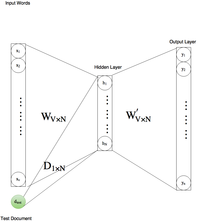
How do we handle new documents in this model? How would one handle new words in word2vec? One solution is to add a new node for this word, find new training data where the new word is present and run some more iterations of W2V training. That is exactly how new documents are handled in P2V. We retrain the model with the words present in the new document (this is the inference step in P2V). Note that the training update equation above doesn’t impact members not in the context set, $\mathcal{C}$. Thus, at inference time model can be seen as below. Also, note that the weights $P$ and $Q$ have already been learnt in the training step and one may choose to treat them as constants at the inference step.

The objective function is same as in negative sampling, repeated here for clarity:

\[f(q_{0},\,\ldots,\,q_{n_i},h) = \log \sigma(q_{j^*}^Th) + \sum_{j\in \mathcal{N}}\log \sigma(-q_j^Th)\]

Update steps treating $P$ and $Q$ constant

$P$ and $Q$ have no updates. Let $d_{test}$ represent the vector representing the new test document.

\[\frac{\partial f}{\partial d_{test}} = \frac{1}{|C|} \frac{\partial f}{\partial h}\]

$\frac{\partial f}{\partial h}$ remains same as above. Update step for this document vector is:

\[d_{test}^{t+1} \leftarrow d_{test}^t + \frac{\eta}{|C|} \sum_j^{\mathcal{N}} e_j q_j\]

Run time for inference is $O(|\mathcal{N}|r)$.

If $P$ and $Q$ are also updated, then the inference step become similar to training and takes $O((|\mathcal{N}|+|\mathcal{C}|)r)$ time.